

Imagine you have got a contact list of a number of leads. You collected it from different sources. So you don’t know if a certain contact is repeating.
All you want is to search by the email and find all the duplicates. I searched around using Google for a quick solution. However I didn’t find a good one. Many of the articles that popped up proposes UNIQUE() formula. I don’t find UNIQUE() useful in this situation. The best function I found useful to highlight duplicates is MATCH(). I will explain the details below.
Get the sample sheet here:
Sample Sheet
When you want to search for duplicates, all it has to do is to search the current cell in all rows before it. Like this:
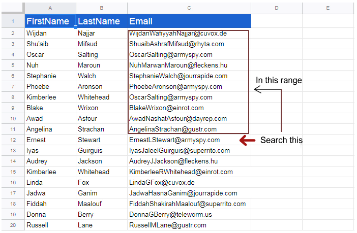
The perfect formula to do this is MATCH()
MATCH(search_key, range, [search_type])
Search key is the value of the current cell and range is the range where to search for
search_type 1 means the range is sorted and search_type 0 means the range is NOT sorted.
The MATCH() function returns the row number where the match is found.
So if we just do
=MATCH( C12, C$2:C11, 0)
The formula will tell us whether the cell C12 has a duplicate (and if there is a duplicate, which row it is)
We can just apply this formula to one cell and just copy to the rest of the cells. Google Sheets will automatically translate the row numbers.
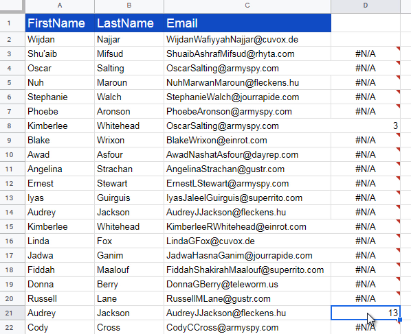
When there is no match, the MATCH() function returns #N/A
It doesn’t look good.
Moreover, notice that in row number 8, it says 3 However, the actual duplicate is in row number 4.
This is because our search range is from row number 2
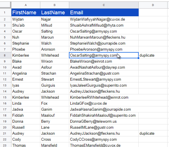
The function to check whether it is N/A is ISNA() combine this with IF() we get this formulat to find duplicates
=IF(ISNA(MATCH(C3,C$2:C2,0)),"","duplicate")
If you spread this formula to the column, it will show you the duplicates
This has one inconvenience that it only tells you that there is a duplicate. It does not tell you where the duplicate is. So we want the row number returned by MATCH() function. Using IF you will have to use MATCH() function twice to get the row number again:
=IF(ISNA(MATCH(C3,C$2:C2,0)),"",MATCH(C3,C$2:C2,0))
But that is ugly and tells low about or Google sheet formula skills 🙂
Here is an alternative:
=SUMIF(MATCH(C3,C$2:C2,0)+1,"#N/A")
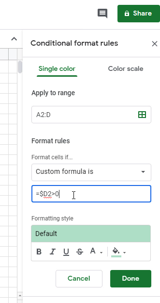
In order to highlight the duplicates, go to menu item : Format → Highlight duplicates
Select range A2:D
Under format rules, select “custom formula is” =$D2 > 0
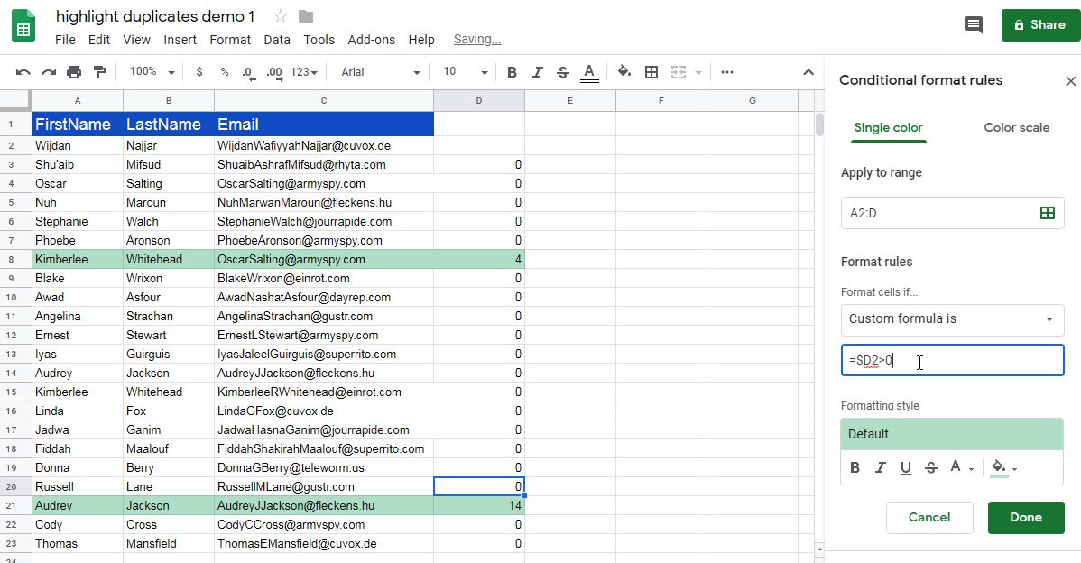
So we have duplicate rows highlighted. Moreover the row number of the duplicate row is readily available. You can filter and delete the duplicate row or use a Query to copy the unique rows to another sheet.
This query gets the unique rows
QUERY(Sheet1!A:D,"Select A,B,C Where D=0")